分位数回归是什么?
分位数回归问的是 X 对 Y 分布不同位置的影响是否不同。OLS 看条件均值,分位数回归可以看低端、中位数和高端样本的条件效应。
先用一句话理解
把 OLS 想成只问平均学生提高多少,分位数回归则分别问后进生、中等生和尖子生提高多少。如果 X 对不同位置的人影响不同,均值会掩盖这种差异。
什么时候用
| 判断项 | 教科书式判断 |
|---|---|
| 适合用在 | 研究关心效应是否在低分位和高分位不同,或因变量分布明显偏态。 |
| 先不要用在 | 只是为了多跑几个分位点找显著,而没有分布异质性问题。 |
| 最关键的前提 | 解释对象是条件分位数,不是无条件分布位置。 |
| 读表顺序 | 先看 τ 是哪个分位点,再比较不同 τ 下系数方向和量级。 |
| 论文表述边界 | 不能把 τ=0.9 的结果写成“高收入个体的因果效应”而不说明条件分位含义。 |
把它和相近方法分清楚
| 容易混淆的对象 | 怎么区分 | 初学者记法 |
|---|---|---|
| OLS | 估计条件均值效应。 | 回答平均水平如何变化。 |
| 分位数回归 | 估计条件分位点效应。 | 回答分布不同位置是否不同。 |
| 异质性分组 | 按可观察组分开估计。 | 分位点不是外生分组。 |
核心直觉和模型公式
条件分位数
τ 分位数回归的对象是:
\[Q_{\tau}(Y_i\mid X_i)=X_i\beta_{\tau}\]
\[\min_{\beta}\sum_i \rho_{\tau}(Y_i-X_i\beta)\]
不同 τ 有不同的 β_τ,所以可以比较低端、中位和高端的条件效应。
公式里的符号怎么读
| 符号 | 含义 | 在本页怎么理解 |
|---|---|---|
| τ | 分位点 | 例如 0.25、0.5、0.75。 |
| Q_τ(Y|X) | 条件分位数 | 给定 X 后 Y 分布的 τ 位置。 |
| β_τ | 分位点系数 | X 对该条件分位点的影响。 |
| ρ_τ | check loss | 分位数回归的非对称损失函数。 |
专业使用口径
分位数回归要写成分布异质性,而不是把多个分位点当多次稳健性搜索。
| 口径 | 专业写法 |
|---|---|
| 分位点选择 | τ 应来自研究问题,常见 0.25/0.5/0.75 或 0.1/0.5/0.9。 |
| 系数比较 | 比较方向、量级和置信区间,而不是只看某个分位点星号。 |
| 标准误 | 通常使用 bootstrap 或稳健标准误。 |
| 解释对象 | 强调条件分位数,不等于固定某个个体处在分布高端。 |
一步一步做:从问题到结果的五步
| 步骤 | 这一页具体做什么 | 做到什么程度才算读懂 |
|---|---|---|
| 1. 说明为什么看分布 | 理论上 X 可能对低端和高端影响不同。 | 没有理由不要机械跑十几个分位点。 |
| 2. 选择分位点 | 预先设定 τ。 | 避免事后挑显著分位。 |
| 3. 估计各 τ 模型 | 同一变量口径下比较 β_τ。 | 样本口径要保持一致。 |
| 4. 画系数路径 | 用图展示 β_τ 随 τ 的变化。 | 单列表格不直观。 |
| 5. 写出异质性 | 说明效应在哪些分位更强或更弱。 | 不要过度解释相邻分位点噪声。 |
结果怎么读:先读口径,再读数字
本页案例读表时,先记住这个口径:0.10 = 0.3934;0.0353。
| 读表顺序 | 本页怎么读 | 不要这样读 |
|---|---|---|
| 先看 τ | 每一列对应哪个条件分位点。 | 不要把 τ 当样本分组标签。 |
| 再看 β_τ | 不同分位点方向和量级是否变化。 | 不要只看星号。 |
| 然后看置信区间 | 分位点之间差异是否足够明显。 | 肉眼差异不等于统计差异。 |
| 最后看理论解释 | 分布异质性是否符合研究机制。 | 不要事后编故事。 |
初学者最容易错在哪里
| 误读 | 为什么错 |
|---|---|
| 把分位点当固定群体 | 错。它是条件分布位置,不是同一批高端个体。 |
| 跑很多 τ 只挑显著 | 错。这会变成多重检验问题。 |
| 把分位数回归当稳健性 | 不准确。它回答的是分布异质性。 |
| 不比较系数路径 | 不够。分位数回归重点在不同 τ 的变化。 |
先看这个案例的结论
- 0.10 = 0.3934;0.0353。
- 0.25 = 0.4928;0.0524。
- 0.50 = 0.6282;0.0556。
- 这些数字来自页面里的结果表;写论文时先解释数值含义,再讨论理论含义。
变量要求和案例口径
| 字段 | 口径 |
|---|---|
| 数据 | CSMAR 风格 A 股企业创新面板 |
| 原始样本 | 196 家上市公司,2015-2020 年,约 1200 个公司-年观测;各方法有效样本以本页输出表 N 为准 |
| 因变量 | patent_count;回归页通常使用 ln(1 + patent_count) |
| 核心解释变量 | dfi_index,数字普惠金融指数;部分案例输出展示的是标准化后的 dfi_index |
| 控制变量 | roa、lev、size、growth、cashflow、tobinq、top1、dual、board、indep、soe、age |
| 输出文件 | quantile_results.csv |
| 角色要求 | 因变量、核心解释变量 |
| 依赖包 | 无额外 Stata 社区包要求 |
实际代码
下面是本页案例里的最小 Stata 代码。它的作用是帮助你看清变量怎么进入模型、结果文件怎么生成,而不是要求你在网页里手动运行。
log using "/root/workspace/empirical-wizard/workspace/2f608d77/analysis.log", replace text
global JOB_DIR "/root/workspace/empirical-wizard/workspace/2f608d77"
set more off
adopath + "/root/ado/plus"
global DATA_PATH "/root/workspace/empirical-wizard/workspace/test_e2e/csmar_innovation.csv"
import delimited "/root/workspace/empirical-wizard/workspace/test_e2e/csmar_innovation.csv", clear case(preserve)
capture confirm global JOB_DIR
if _rc global JOB_DIR "."
* 自动去除完全重复行(同列同值),避免 N 虚增与 xtset 失败
quietly duplicates drop
local idvar ""
local timevar ""
capture confirm variable stkcd
if !_rc {
    capture confirm numeric variable stkcd
    if _rc {
        tempvar __ewiz_id
        capture encode stkcd, gen(`__ewiz_id')
        if !_rc local idvar "`__ewiz_id'"
    }
    else {
        local idvar "stkcd"
    }
}
else {
    di as text "面板ID变量不存在,跳过 xtset ID:stkcd"
}
capture confirm variable year
if !_rc {
    capture confirm numeric variable year
    if _rc {
        tempvar __ewiz_time
        capture encode year, gen(`__ewiz_time')
        if !_rc local timevar "`__ewiz_time'"
    }
    else {
        local timevar "year"
    }
}
else {
    di as text "时间变量不存在,跳过 xtset time:year"
}
if "`idvar'" != "" & "`timevar'" != "" {
    capture xtset `idvar' `timevar'
}

* ── 分位数回归 ──
tempname fh
capture file close `fh'
file open `fh' using "$JOB_DIR/quantile_results.csv", write replace
file write `fh' "分位数,系数,标准误,t/z 值,p 值,95% CI 下限,95% CI 上限,N" _n

* 分位数 0.10
capture noisily qreg patent_count dfi_index roa lev size growth cashflow tobinq top1 dual board indep soe age, quantile(0.1) vce(robust)
if !_rc {
    local _coef : display %9.4f _b[dfi_index]
    local _se : display %9.4f _se[dfi_index]
    local _t = _b[dfi_index] / _se[dfi_index]
    local _p : display %9.4f 2*ttail(e(df_r), abs(`_t'))
    local _t : display %7.3f `_t'
    local _cil : display %9.4f _b[dfi_index] - 1.96 * _se[dfi_index]
    local _cih : display %9.4f _b[dfi_index] + 1.96 * _se[dfi_index]
    local _n = e(N)
    file write `fh' "0.10,`_coef',`_se',`_t',`_p',`_cil',`_cih',`_n'" _n
}
else {
    file write `fh' "0.10,.,.,.,.,.,.,." _n
}

* 分位数 0.25
capture noisily qreg patent_count dfi_index roa lev size growth cashflow tobinq top1 dual board indep soe age, quantile(0.25) vce(robust)
if !_rc {
    local _coef : display %9.4f _b[dfi_index]
    local _se : display %9.4f _se[dfi_index]
    local _t = _b[dfi_index] / _se[dfi_index]
    local _p : display %9.4f 2*ttail(e(df_r), abs(`_t'))
    local _t : display %7.3f `_t'
    local _cil : display %9.4f _b[dfi_index] - 1.96 * _se[dfi_index]
    local _cih : display %9.4f _b[dfi_index] + 1.96 * _se[dfi_index]
    local _n = e(N)
    file write `fh' "0.25,`_coef',`_se',`_t',`_p',`_cil',`_cih',`_n'" _n
}
else {
    file write `fh' "0.25,.,.,.,.,.,.,." _n
}

* 分位数 0.50
capture noisily qreg patent_count dfi_index roa lev size growth cashflow tobinq top1 dual board indep soe age, quantile(0.5) vce(robust)
if !_rc {
    local _coef : display %9.4f _b[dfi_index]
    local _se : display %9.4f _se[dfi_index]
    local _t = _b[dfi_index] / _se[dfi_index]
    local _p : display %9.4f 2*ttail(e(df_r), abs(`_t'))
    local _t : display %7.3f `_t'
    local _cil : display %9.4f _b[dfi_index] - 1.96 * _se[dfi_index]
    local _cih : display %9.4f _b[dfi_index] + 1.96 * _se[dfi_index]
    local _n = e(N)
    file write `fh' "0.50,`_coef',`_se',`_t',`_p',`_cil',`_cih',`_n'" _n
}
else {
    file write `fh' "0.50,.,.,.,.,.,.,." _n
}

* 分位数 0.75
capture noisily qreg patent_count dfi_index roa lev size growth cashflow tobinq top1 dual board indep soe age, quantile(0.75) vce(robust)
if !_rc {
    local _coef : display %9.4f _b[dfi_index]
    local _se : display %9.4f _se[dfi_index]
    local _t = _b[dfi_index] / _se[dfi_index]
    local _p : display %9.4f 2*ttail(e(df_r), abs(`_t'))
    local _t : display %7.3f `_t'
    local _cil : display %9.4f _b[dfi_index] - 1.96 * _se[dfi_index]
    local _cih : display %9.4f _b[dfi_index] + 1.96 * _se[dfi_index]
    local _n = e(N)
    file write `fh' "0.75,`_coef',`_se',`_t',`_p',`_cil',`_cih',`_n'" _n
}
else {
    file write `fh' "0.75,.,.,.,.,.,.,." _n
}

* 分位数 0.90
capture noisily qreg patent_count dfi_index roa lev size growth cashflow tobinq top1 dual board indep soe age, quantile(0.9) vce(robust)
if !_rc {
    local _coef : display %9.4f _b[dfi_index]
    local _se : display %9.4f _se[dfi_index]
    local _t = _b[dfi_index] / _se[dfi_index]
    local _p : display %9.4f 2*ttail(e(df_r), abs(`_t'))
    local _t : display %7.3f `_t'
    local _cil : display %9.4f _b[dfi_index] - 1.96 * _se[dfi_index]
    local _cih : display %9.4f _b[dfi_index] + 1.96 * _se[dfi_index]
    local _n = e(N)
    file write `fh' "0.90,`_coef',`_se',`_t',`_p',`_cil',`_cih',`_n'" _n
}
else {
    file write `fh' "0.90,.,.,.,.,.,.,." _n
}

file close `fh'

* coef-by-quantile plot via grqreg if available — only on small/mid samples
quietly count if !missing(patent_count)
local __sqreg_n = r(N)
local __sqreg_reps = 200
if `__sqreg_n' > 30000 local __sqreg_reps = 100
if `__sqreg_n' > 100000 {
    di as text "sqreg skipped: N=`__sqreg_n' too large for simultaneous-quantile bootstrap; the five separate qreg runs above already provide the per-quantile coefficients."
}
else {
    capture noisily sqreg patent_count dfi_index roa lev size growth cashflow tobinq top1 dual board indep soe age, q(0.1 0.25 0.5 0.75 0.9) reps(`__sqreg_reps')
    capture which grqreg
    if !_rc {
        capture noisily grqreg dfi_index, ci ols olsci
        capture graph export "$JOB_DIR/quantile_coef_plot.png", replace width(1800)
    }
}

di "分位数回归完成 (5 个分位数)"
log close
实际输出表
这张表是本方法页配套案例的输出结果,用来把前面的公式、变量口径和代码对应到实际数字。
| 分位数 | 系数 | 标准误 | t/z 值 | p 值 | 95% CI 下限 | 95% CI 上限 | N |
|---|---|---|---|---|---|---|---|
| 0.10 | 0.3934 | 0.0353 | 11.152 | 0.0000 | 0.3243 | 0.4626 | 720 |
| 0.25 | 0.4928 | 0.0524 | 9.398 | 0.0000 | 0.3900 | 0.5956 | 720 |
| 0.50 | 0.6282 | 0.0556 | 11.296 | 0.0000 | 0.5192 | 0.7373 | 720 |
| 0.75 | 0.5981 | 0.0442 | 13.525 | 0.0000 | 0.5115 | 0.6848 | 720 |
| 0.90 | 0.5896 | 0.0563 | 10.471 | 0.0000 | 0.4792 | 0.6999 | 720 |
案例图
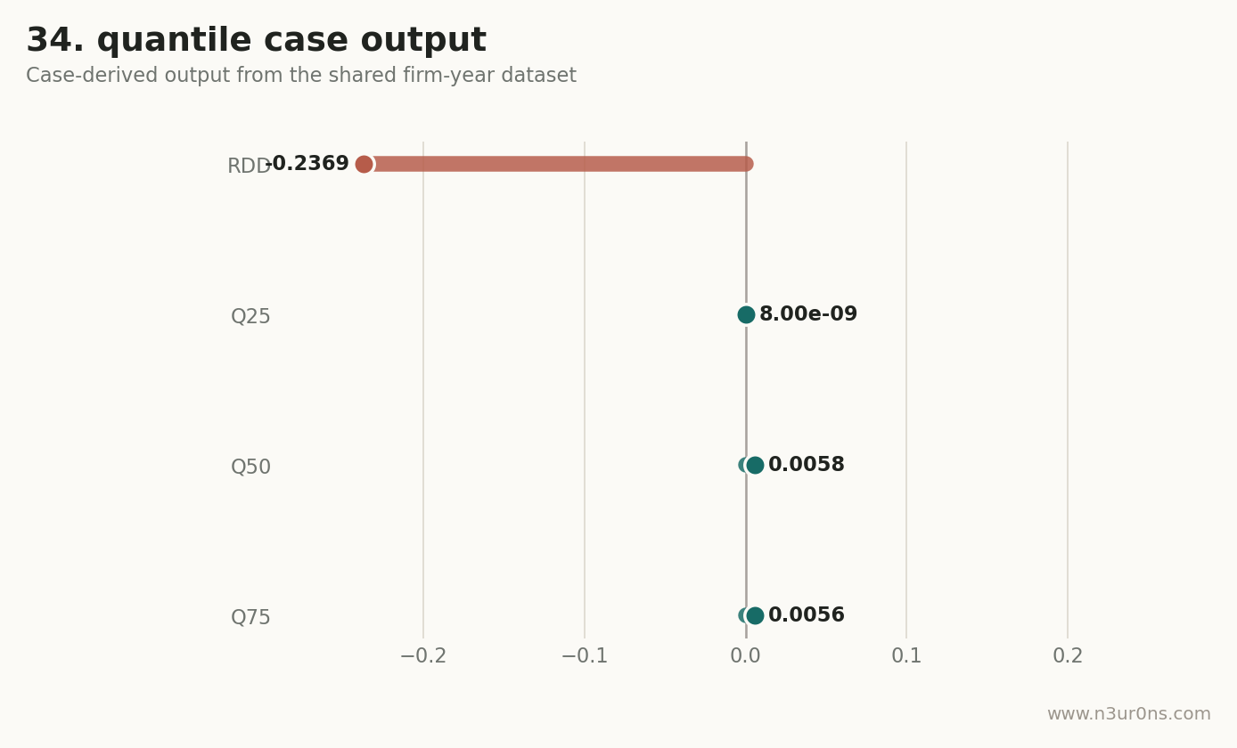
这是一张由同一份案例数据生成的页面内诊断图。
论文里怎么写
本文在共用企业面板样本上报告分位数回归,核心输出见 quantile_results.csv。结果解释时同时关注样本口径、变量构造、系数方向、标准误和适用前提,避免只凭单个 p 值完成方法选择。
检查清单
- 先说明为什么均值效应不够,需要看低分位、中位或高分位。
- 不同分位点的系数要分别解释,不能把它们平均成一个主效应。
- 分位数结果应关注分布异质性,而不是只找哪个分位显著。